- Real-Time Graphics |
- Rendering |
- Animation |
- Geometric Modeling |
- Scientific Visualization |
- Software System

- Chemical Kinetics-Assisted, Path-Based Smoke Simulation

- Animation of Chemically Reactive Fluids Using a Hybrid Simulation Method

- Practical Animation of Turbulent Splashing Water

- View-Dependent Adaptive Animation of Liquids

- Controllable Local Monotonic Cubic Interpolation in Fluid Animations

- Animation of Reactive Gaseous Fluids through Chemical Kinetics

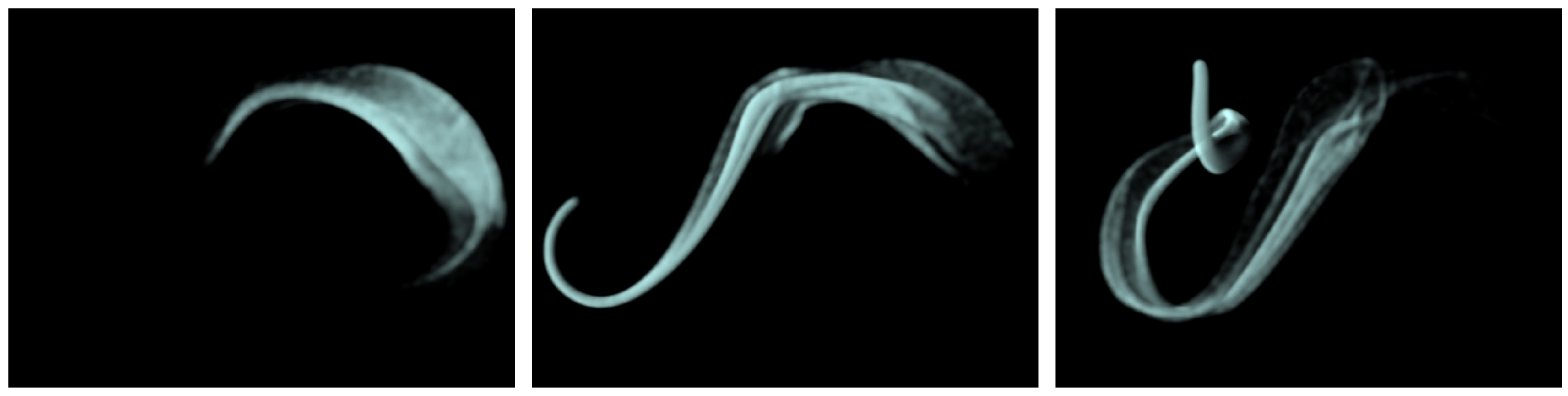
Despite recent successes in physics-based fluid animation, generating desired fluid flow with intuitive control of its motion still remains a challenging problem in the special effects industry. In this paper, we propose a novel approach for path-based smoke simulation that explores the theory of chemical kinetics in an aim to provide a useful animation tool. By describing intended smoke effects through chemical reaction equations and adjusting their parameters, our method allows to easily create various interesting smoke effects that were often hard to get with previous techniques.
To demonstrate the effectiveness of the presented animation framework, we describe several examples of path-based smoke animations, generated with easily understandable reaction equations and control parameters.
- Y. Jang and I. Ihm, "Chemical Kinetics-Assisted, Path-Based Smoke Simulation," Computer Animation and Virtual Worlds (The 22nd Annual Conference on Computer Animation and Social Agent), Vol. 20, No. 2-3, pp. 247-256, June 2009.
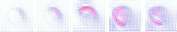
- A two-dimensional slice of induced velocity fields (Figure 3).
- Control with reaction parameters I (Figure 4).
 (a) Using the stoichiometric coefficient
λ2(λ2= 0.5, 1.5, and 2.0)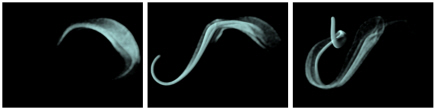 (b) Using the molar masse M
D(MD= 0.2, 0.1, and 0.05) - Control with reaction parameters II (Figure 5).

 (a) Using the two coefficients γ
1and γ2in the first reaction equation
((γ1, γ2) = (300, 0.5) and (300, 2.0))
 (b) Using the coefficient ε
Pin the divergence adjustment function
(εP= 1.0 and 1.5) - Four path-based smoke animation effects (Figure 6).
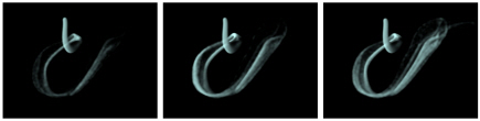
 (a) Disappearing and reappearing smoke
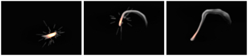 (b) Splashing smoke with instant glows
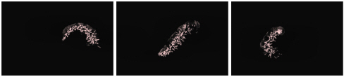 (c) Repeatedly splashing smoke
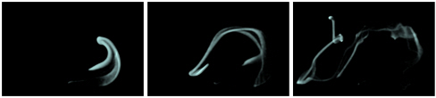
 (d) Smoke and soot
 - More examples (Figure 7).
 (a) The 'fluid' scene before rendering
 (b) The 'fluid' scene after rendering
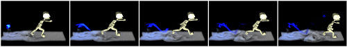 (c) The 'running man' scene


- A two-dimensional slice of induced velocity fields (Figure 3). View
- Control with reaction parameters I (Figure 4).
(a) Using the stoichiometric coefficient λ2(λ2= 0.5, 1.5, and 2.0) View
(b) Using the molar masse MD(MD= 0.2, 0.1, and 0.05) View - Control with reaction parameters II (Figure 5).
(a) Using the two coefficients γ1and γ2in the first reaction equation
((γ1, γ2) = (300, 0.5) and (300, 2.0)) View
(b) Using the coefficient εPin the divergence adjustment function
(εP= 1.0 and 1.5) View - Four path-based smoke animation effects (Figure 6).
(a) Disappearing and reappearing smoke View
(b) Splashing smoke with instant glows View
(c) Repeatedly splashing smoke View
(d) Smoke and soot View - More examples (Figure 7).
(a) The 'fluid' scene before rendering View
(b) The 'fluid' scene after rendering View
(c) The 'running man' scene View
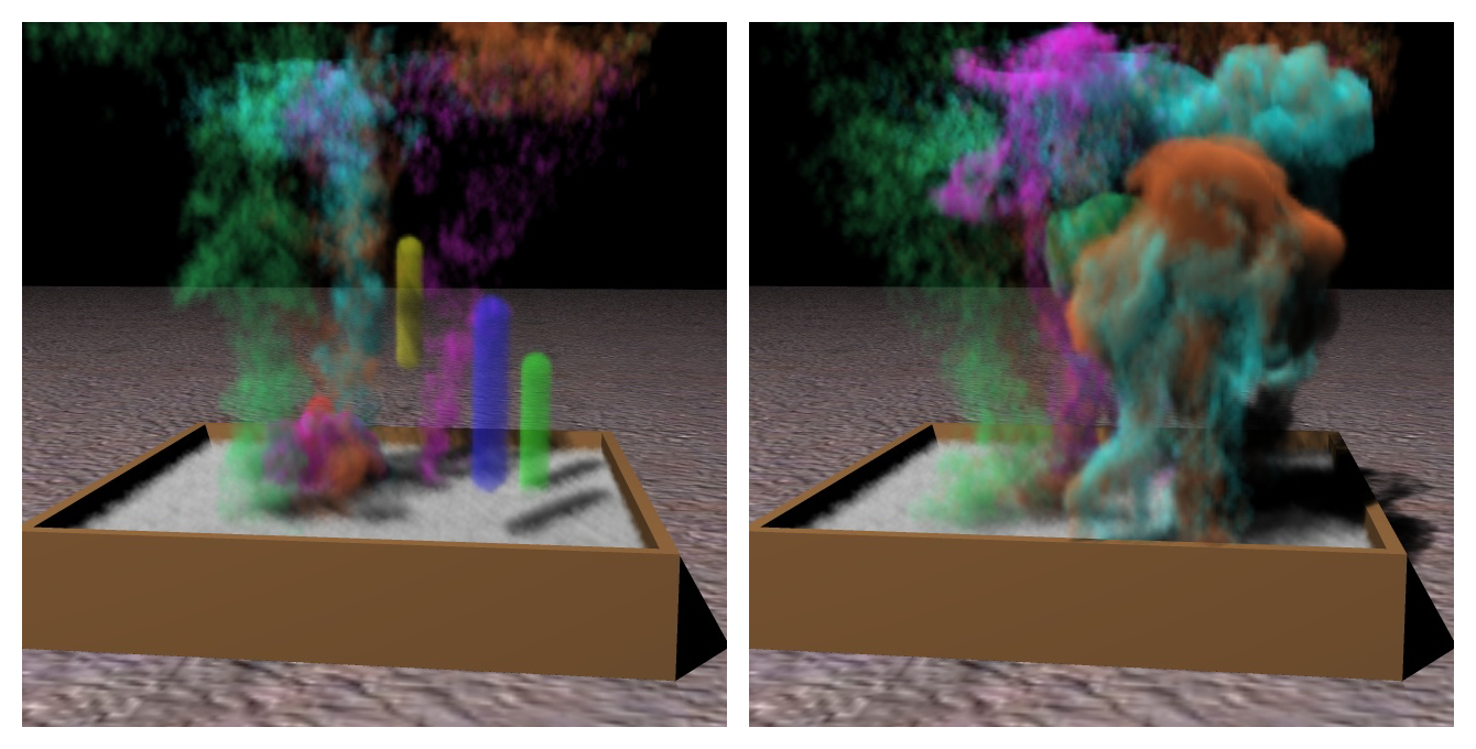
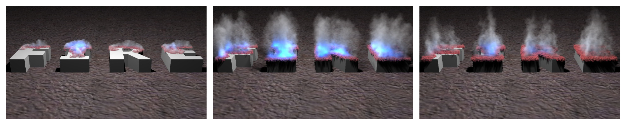
Chemical phenomena abound in the real world, and often comprise indispensable elements of visual effects that are routinely created in the film industry. In this paper, we present a hybrid technique for simulating chemically reactive fluids, based on the theory of chemical kinetics. Our method makes synergistic use of both Eulerian grid-based methods and Lagrangian particle methods to simulate real and hypothetical chemical mechanisms effectively and efficiently. We demonstrate that by modeling chemical reactions using a particle system, an established, physically based fluid system can be extended easily to generate a wide range of chemical phenomena, ranging from catalysis and erosion to fire and explosions, with only a small additional cost.
- B. Kang, Y. Jang, and I. Ihm, "Animation of Chemically Reactive Fluids Using a Hybrid Simulation Method," ACM SIGGRAPH/Eurographics Symposium on Computer Animation, pp. 199-208, San Diego, U.S.A., August 2007
- Hybrid representation of a reaction mechanism.
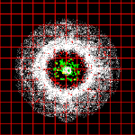
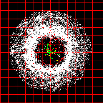
- Particles used in the simulation.
 Material and vortex particles
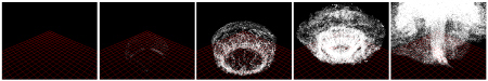 Soot particles
 - Soot particles in rendering.
- Particle-based simulation of a chemical reaction.
 One-step integration
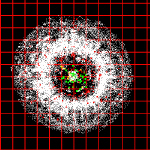 Three-step integration
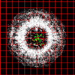 Five-step integration
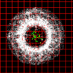 Ten-step integration
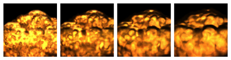
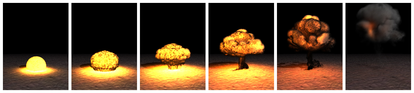
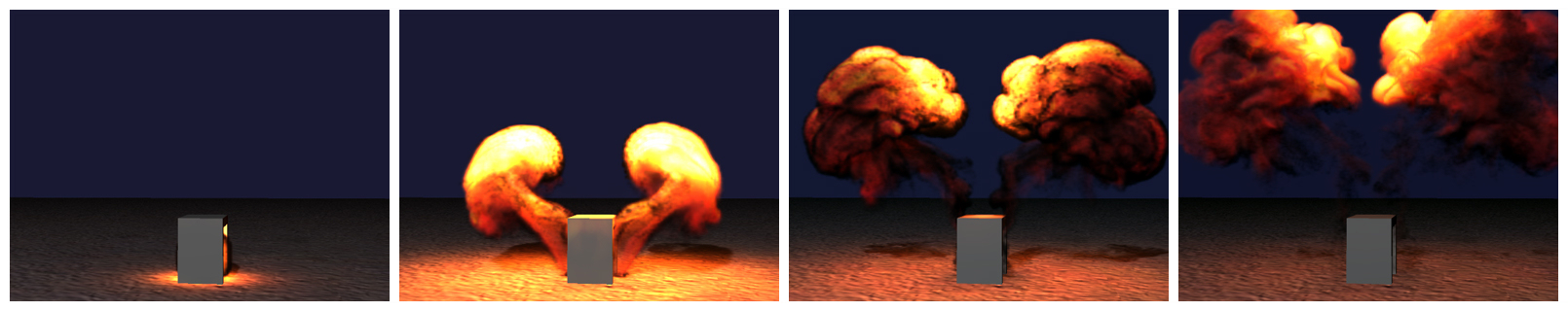
 - Examples of animation scenes.
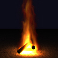
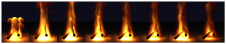 Campfire scene
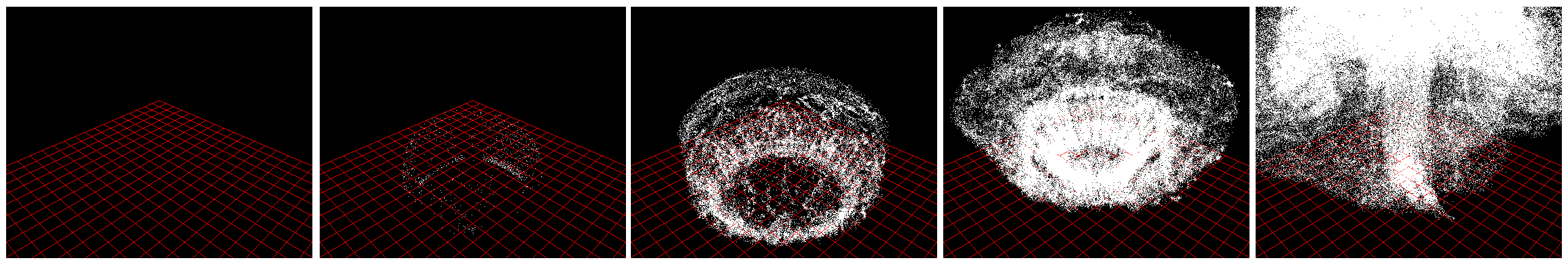
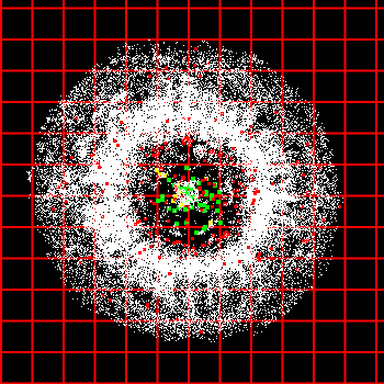
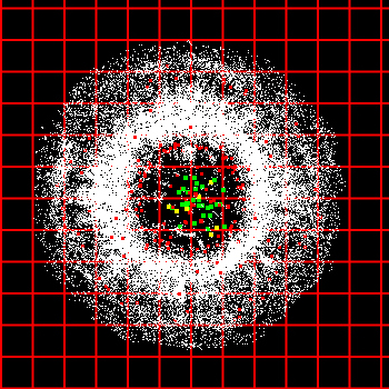
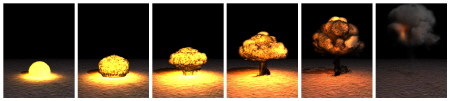 Explosion scene 1
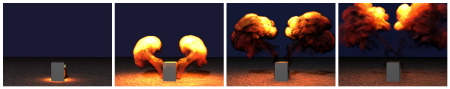 Explosion scene 2
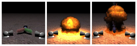 Explosion scene 3
 Eleven species scene
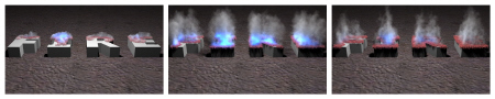 Catalysis scene 1
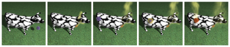 Catalysis scene 2
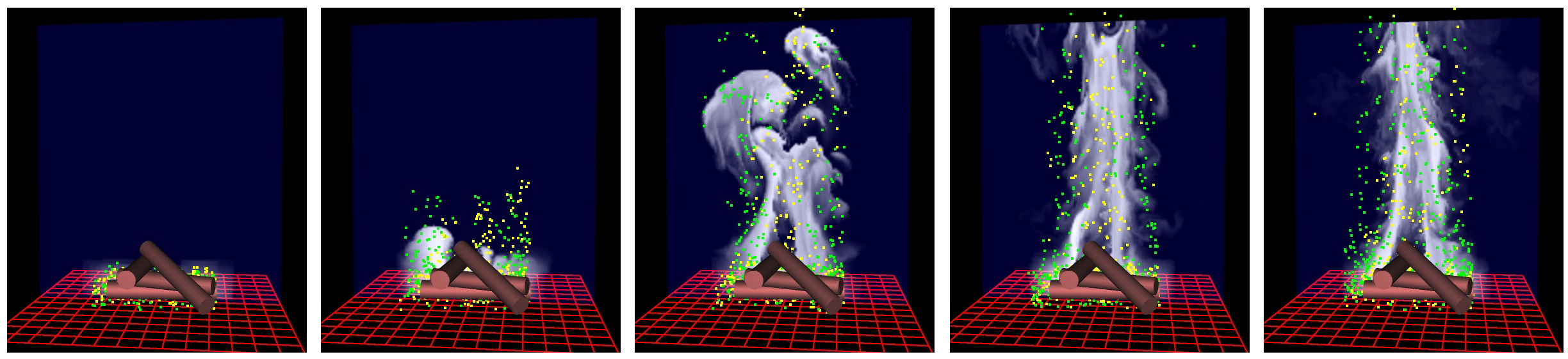


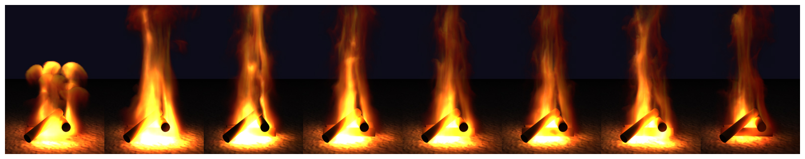


- Hybrid representation of the reaction mechanism for the campfire scene View
- Particles in the simulation of the explosion scene 1 View
- Campfire scene View
- Explosion scene 1 View
- Explosion scene 2 View
- Explosion scene 3 View
- Eleven species scene View
- Catalysis scene 1 View
- Catalysis scene 2 View
- [pdf]
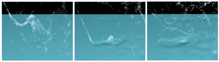
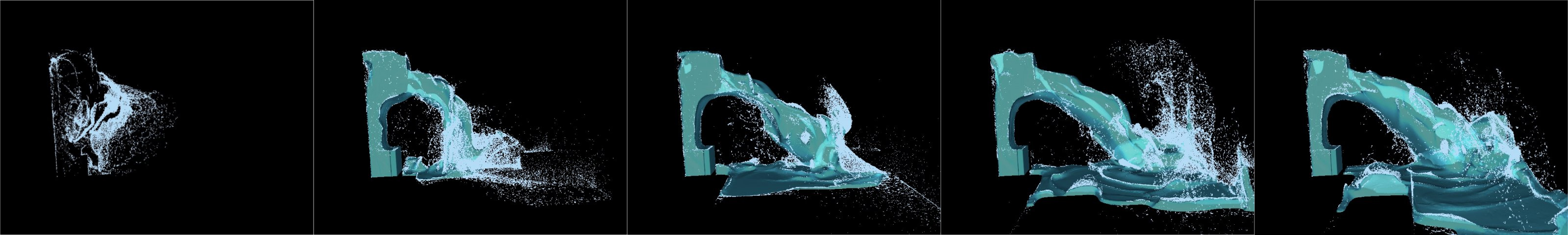
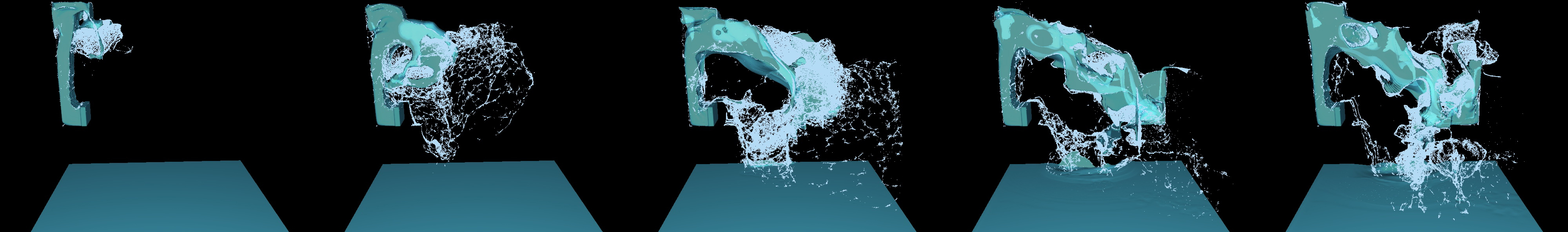
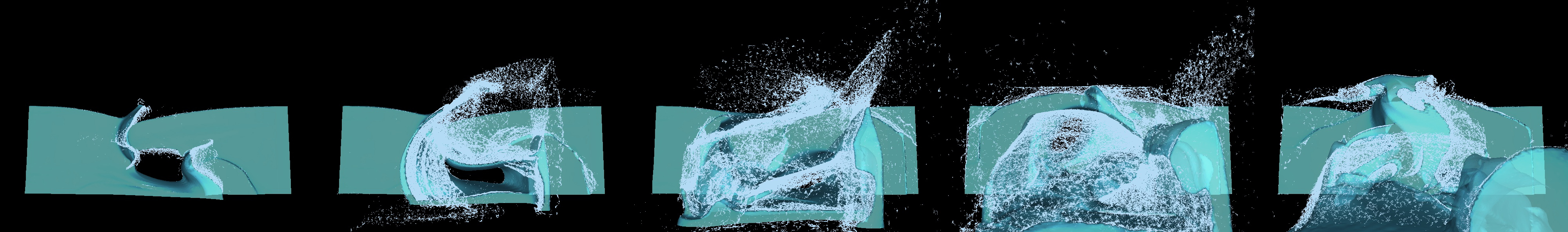
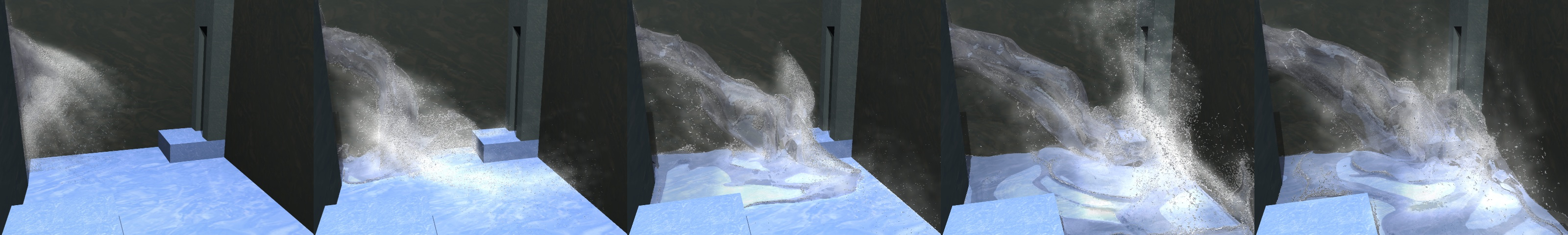
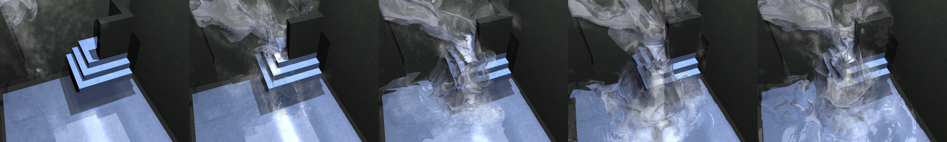
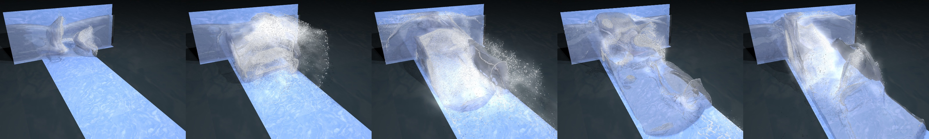
Despite recent advances in fluid animation, producing small-scale detail of turbulent water still remains challenging. In this paper, we extend the well-accepted particle level set method in an attempt to integrate the dynamic behavior of splashing water easily into a fluid animation system. Massless marker particles that still escape from the main body of water, in spite of the level set correction, are transformed into water particles to represent subcell-level features that are hard to capture with a limited grid resolution. These physical particles are then moved in the air through a particle simulation system that, combined with the level set, creates realistic turbulent splashing. In the rendering stage, the particle's physical properties such as mass and velocity are exploited to generate a natural appearance of water droplets and spray. In order to visualize the hybrid water, represented in both level set and water particles, we also extend a Monte Carlo ray tracer so that the particle agglomerates are smoothed, thickened, if necessary, and rendered efficiently. The effectiveness of the presented technique is demonstrated with several examples of pictures and animations.
- J. Kim, D. Cha, B. Chang, B. Koo, I. Ihm, "Practical Animation of Turbulent Splashing Water", ACM SIGGRAPH/Eurographics Symposium on Computer Animation, pp. 335-344, Vienna, Austria, September 2006
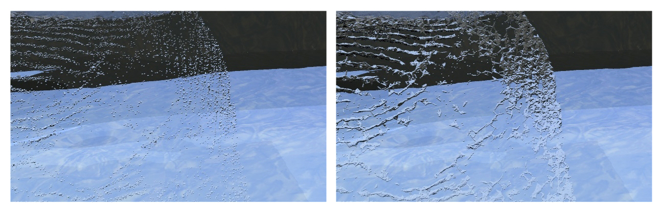
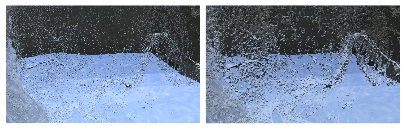
- Impact of falling droplets on water surface.
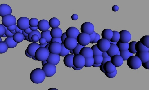
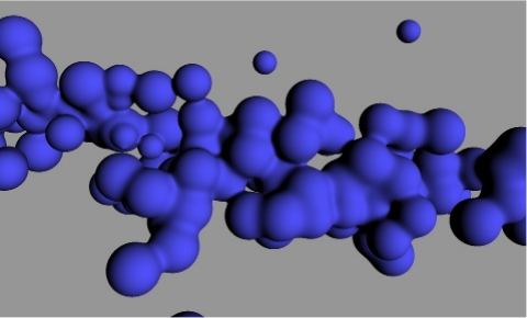
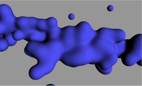
- Smoothing of clusters of spheres.
 A particle cluster
 Blended with �� = 1.5
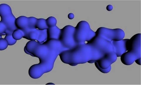
 Blended with �� = 2.0
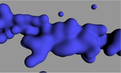 Blended with �� = 2.5
 - Examples of the smoothing and thickening effects
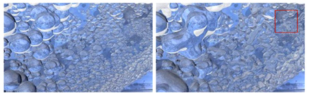 Before and after smoothing 1
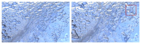 Before and after smoothing 2
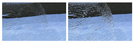 Before and after thickening 1
 Before and after thickening 2
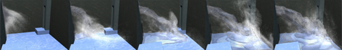
 - Simulation results.
 Scene 1: Pouring water in the room
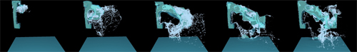 Scene 2: Pouring water onto the stairs.Scene 3: Flood in the corridor.
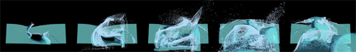 Scene 3: Flood in the corridor - another view.
 - Rendering results.
 Scene 1: Pouring water in the room
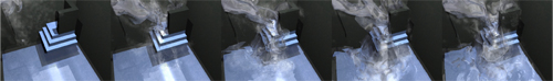 Scene 2: Pouring water onto the stairs.
 Scene 3: Flood in the corridor.
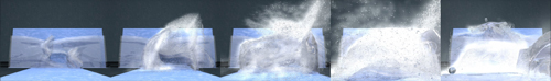 Scene 3: Flood in the corridor - another view.

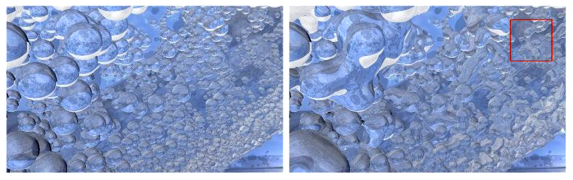


- Before and after smoothing View
- Before and after thickening View
- After adding spray View
- Scene 1: Pouring water in the room View
- Scene 2: Pouring water onto the stairs View
- Scene 3: Flood in the corridor View
- Scene 3: Flood in the corridor - another view View
- [pdf]
Various adaptive mesh refinement techniques are often employed in numerical simulations for increasing spatial and temporal resolution beyond the limits imposed by available CPU time and memory space. Recently, an octree-based adaptive mesh structure was successfully used in fluid animation to place more grid cells efficiently in visually interesting regions of fluids. In an attempt to optimize the use of computational resources further in fluid animation, this paper extends this adaptive technique by modifying the mesh refinement scheme so that the camera's viewing properties are dynamically exploited during the simulation. Based on a simple adaptive mesh structure, we show that the new meshing strategy can save a substantial amount of computation time and memory space by using a view-dependent adaptive approach. The experimental results reveal that the proposed technique provides a good compromise between the computational effort and the simulation's fidelity, and may be used quite effectively in 3D animation production.
- J. Kim, I. Ihm, and D. Cha, "View-Dependent Adaptive Animation of Liquids," ETRI Journal, Vol. 28, No. 6, pp. 697-708, December, 2006
- Liquid animation in a large simulation domain, discretized using a
 grid. Such a grid resolution is still a burden, even to the latest computer, when the simulation is carried out naively. Exploiting the fact that the camera sees only a small portion of the entire domain in each frame, we extended the idea of the adaptive simulation technique so that relatively more refined mesh elements are placed inside the camera's viewing volume. The sequence in the bottom row shows the corresponding scenes, seen from the camera, which were simulated using our view-dependent adaptive method. With the view-dependent adaptive approach, only a
  symmetric linear system with 1,610,592 nonzero elements, on average, must be inverted to solve the Poisson equation in each time step. This implies a remarkable saving considering that a
  linear system with 8,071,956 nonzero elements must be solved in each time step when the simulation is performed on a fixed, uniform grid of smaller resolution,
  .
.
210_click.jpg)
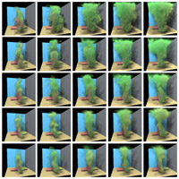
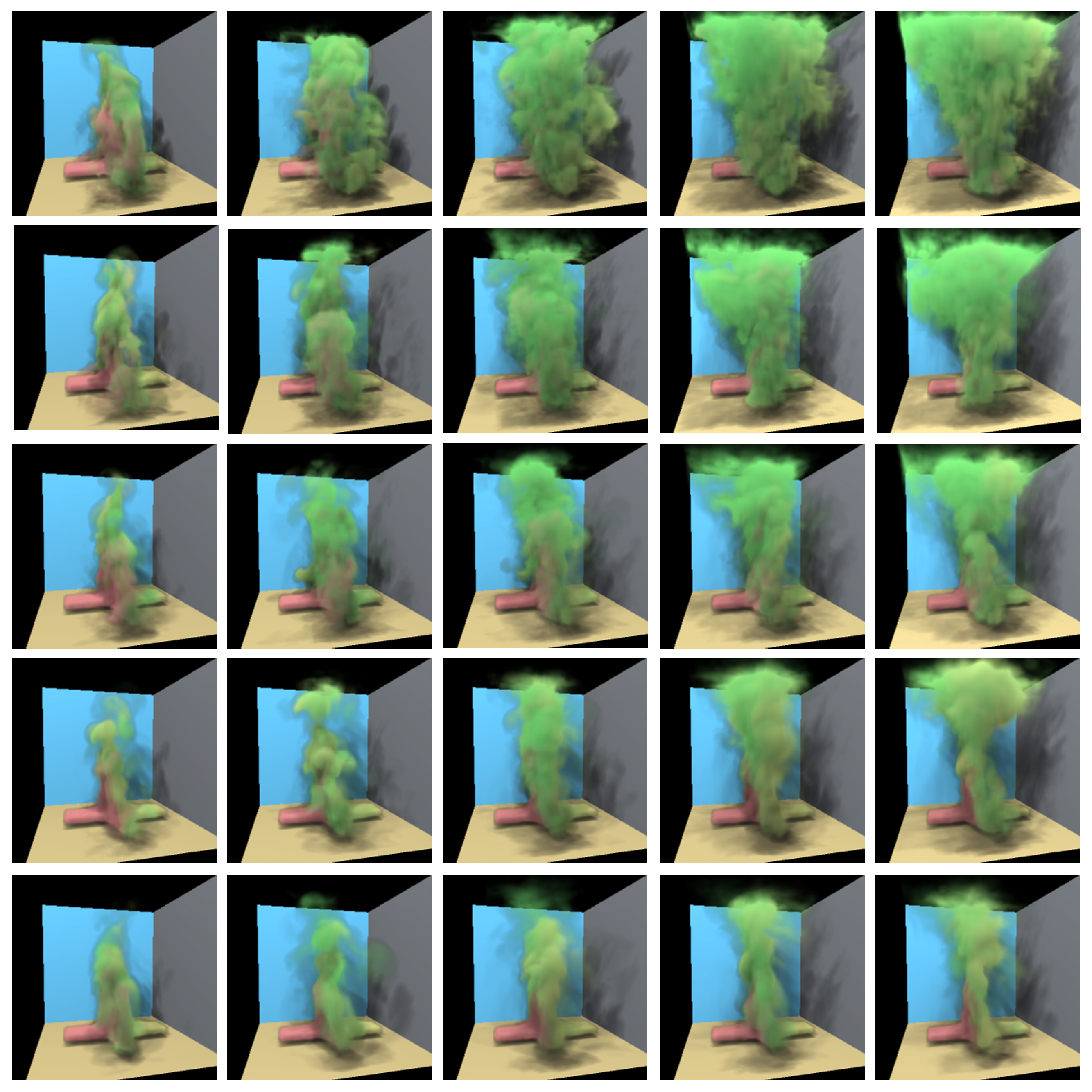
- Animation sequences comparing the three simulation schemes (frame nos.: 40, 90, 160, 210, 400). The first three rows show snapshots of the entire computational domain in the order of
 ,
,  , and
, and  , respectively, while the remaining rows illustrate the corresponding views taken from the moving camera. The effective resolution achieved in this experiment is .
225_click.jpg)
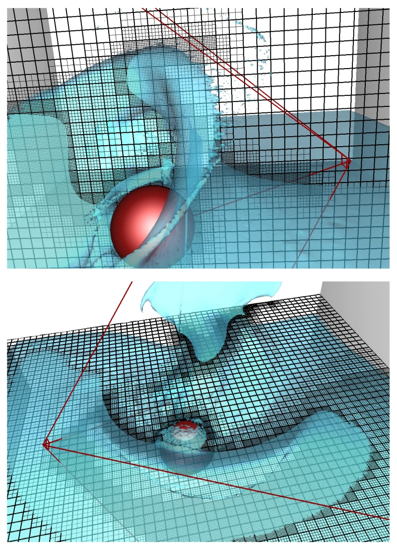
- Two examples of the view-dependent mesh refinement. These pictures show two snapshots of the view-dependent simulation where the orthogonal cutting planes reveal how the computational resources are allocated considering the view information.
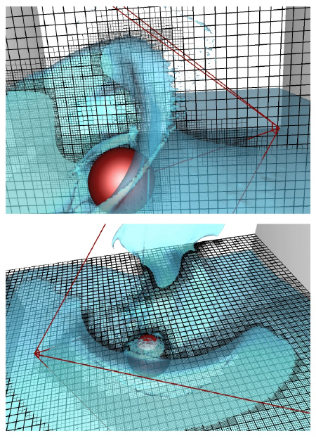
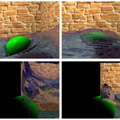
- Two sample snapshots illustrating the effect of the view-dependent refinement. For rendering, we located the rendering camera slightly behind the actual camera. The area colored in red represents the back of the camera, while the uncolored area corresponds to the front-most region of the viewing volume to which the heaviest computing resources~(level 3 refinement) are allocated. The next region in the viewing volume is colored in green where level 2 refinement was applied~(the green region appears in the video). Clearly, the surface details are depicted well in the front-most part, and the details gradually disappear at the back of the camera.
800_click.jpg)
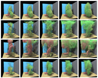
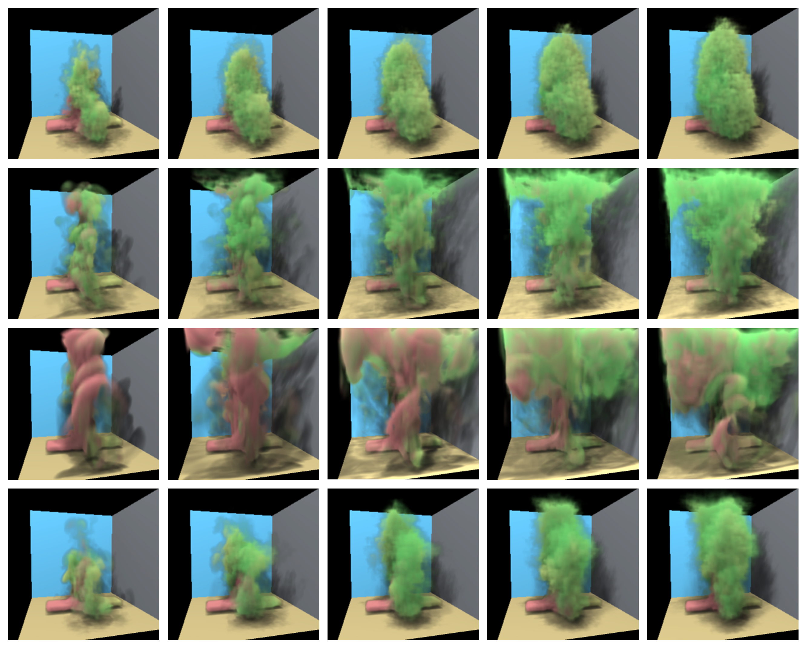
- Animation sequences comparing the two adaptive simulation schemes~(frame nos.: 100, 200, 300, ... , 1000). Again, the entire computational domain and the views taken from the actual camera are demonstrated for and , respectively. The effective resolution applied in this experiment is
 . Although the numerical errors introduced by the view-dependent computing are accumulated additional to those caused by the adaptive mesh refinement, this experiment shows that a clever allocation of CPU time and memory space may lead to an effective view-dependent adaptive simulation technique quite suitable for 3D animation production.
200_click.jpg)
210.jpg)
225.jpg)
800.jpg)
200.jpg)
- Test scene I (effective resolution: )
- Simulation on a fixed grid
Entire Scene / From Camera - Octree-based adaptive simulation
Entire Scene / From Camera - View-dependent adaptive simulation
Entire Scene / From Camera
- Simulation on a fixed grid
- Test scene II (effective resolution: )
- Octree-based adaptive simulation
Entire Scene / From Camera - View-dependent adaptive simulation
Entire Scene / From Camera / From camera (level display)
- Octree-based adaptive simulation
- Test scene III (effective resolution: )
- View-dependent adaptive simulation
Entire Scene / From Camera
- View-dependent adaptive simulation
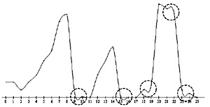
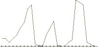
- Frame-by-frame Matrix size required to solve the Poisson equation.
While linear interpolation has been used frequently in computer graphics, higher-order interpolation is often desirable in applications requiring higher-order accuracy. In this paper, we study how interpolation filters, employed to resample such data as velocity, density, and temperature in simulating the equations of fluid dynamics, affect the animation of fluids. For this purpose, we have designed a controllable local cubic interpolation scheme that offers  (or
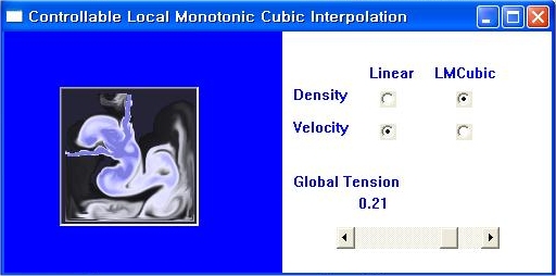
(or  ) continuity globally. It is based on monotonic splines so does not suffer from undue overshooting. Furthermore, it is possible to control the general behavior of the interpolation through a global tension parameter, providing a continuous spectrum of linear to cubic interpolation. We analyze how this controllable interpolation filter may be effectively used to enhance the visual reality for physically based fluid animation.
- I. Ihm, D. Cha, and B. Kang, "Controllable Local Monotonic Cubic Interpolation in Fluid Animations", Computer Animation and Virtual Worlds, October 2005.
- An example of cubic interpolation
 before monotonicity is enforced
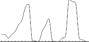 after monotonicity is enforced with
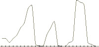
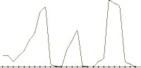
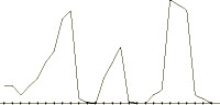
- A spectrum of controllable monotonic cubic interpolants


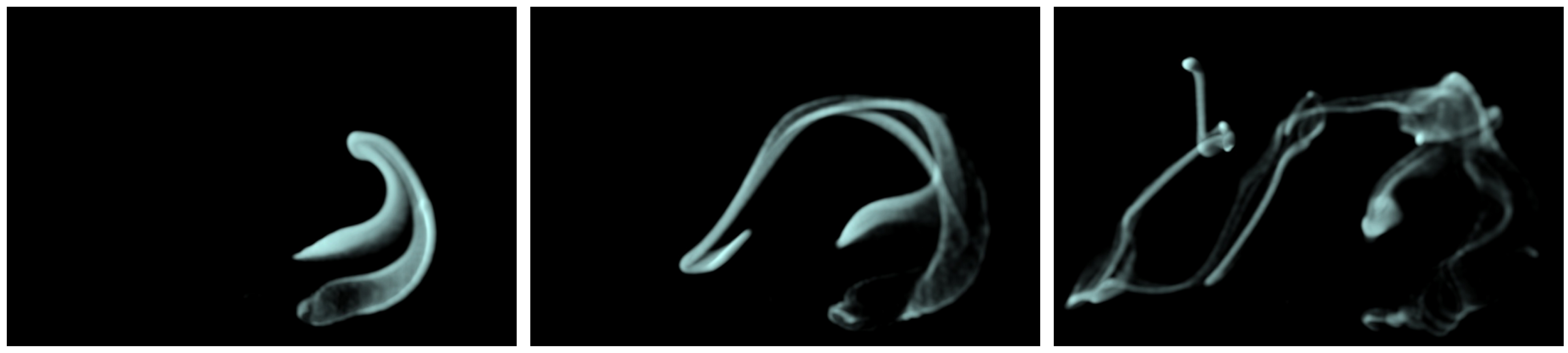
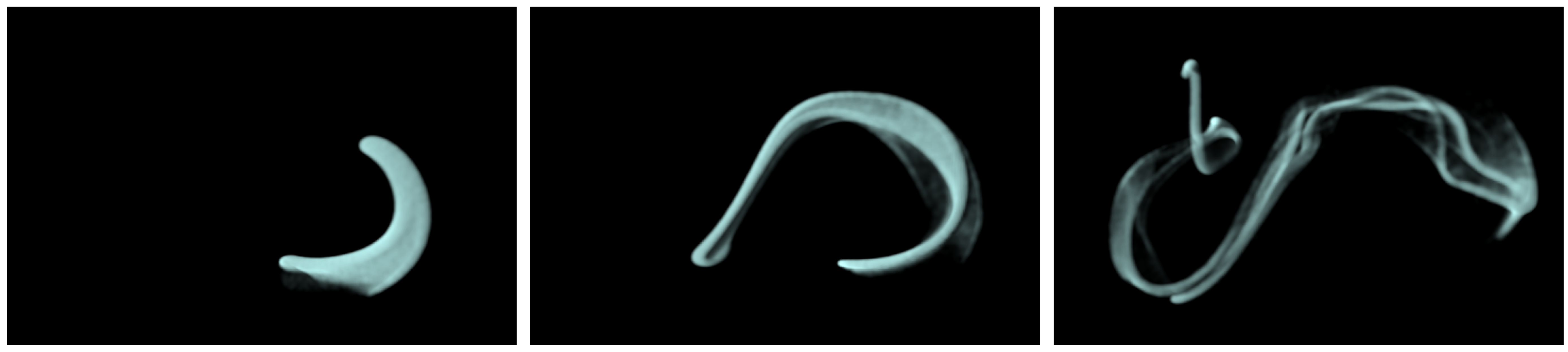
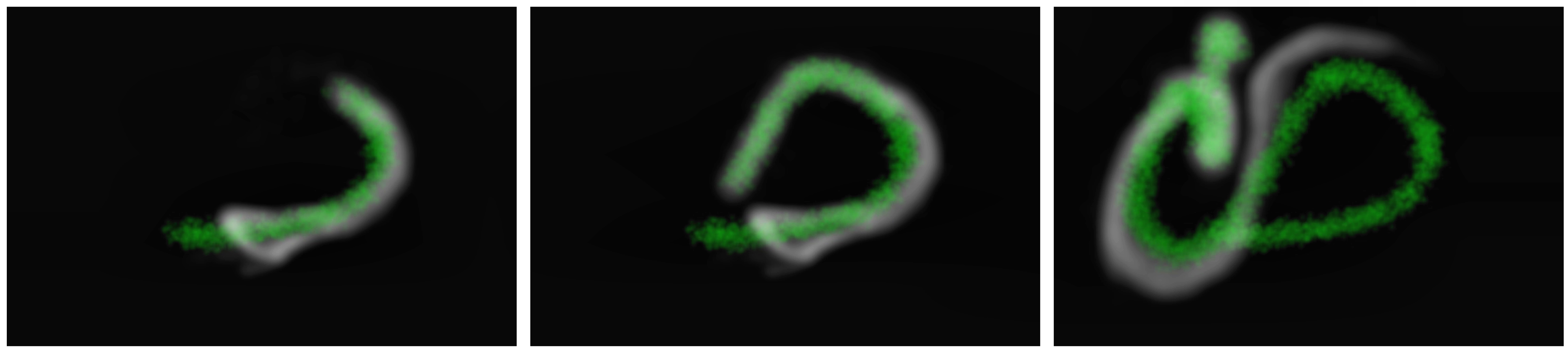
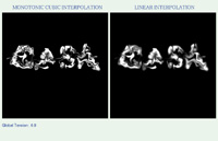
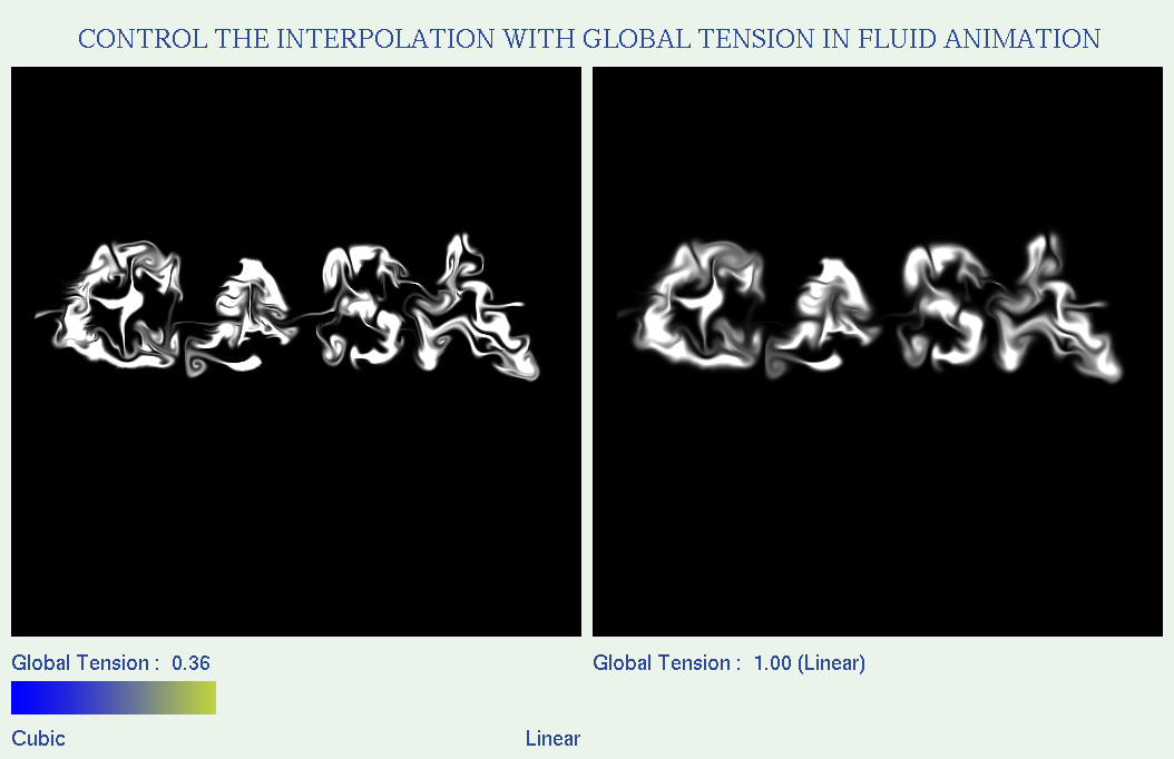
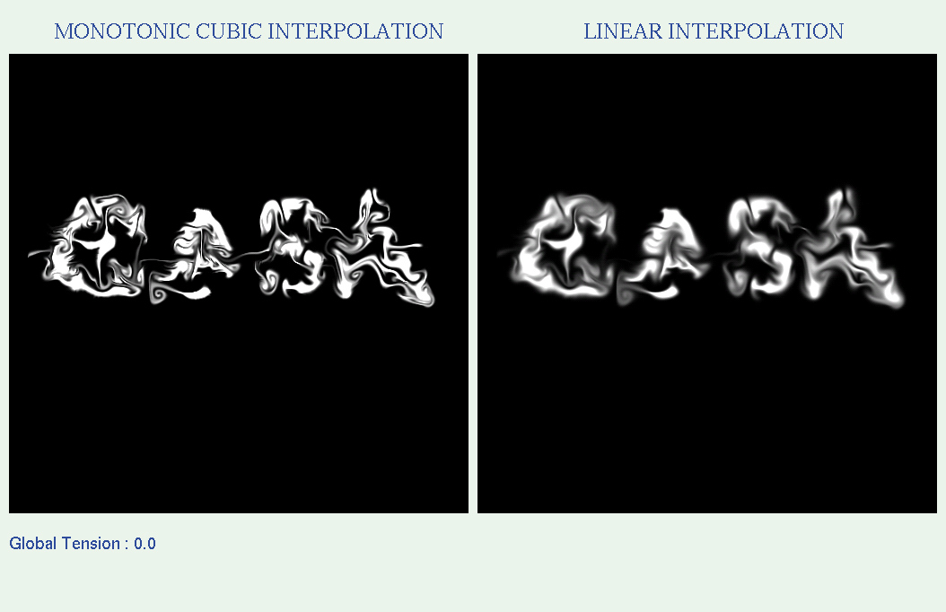
- Comparison of rising-and-reacting smokes created with our local monotonic cubic interpolants
 = 0.0, 0.25, 0.50, 0.75, and 1.0
 - Comparison of rising-and-reacting smoke created by additionally applying our local monotonic cubic interpolant to the velocity resampling
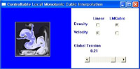
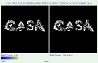
- Interactive control of the global tension parameter
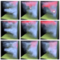
- Application to smoke control
- Image 3 : [first row], [second row], [third row], [fourth row], [fifth row]
- Image 4 : [first row], [second row], [third row], [fourth row]
- Image 5 : [click]
- Image 6 : [left], [right]
Although chemically reactive fluids may be used effectively to increase the reality of visual effects, little work has been done with the general modeling of chemical reactions in computer animation. In this paper, we attempt to extend an established, physically based fluid simulation technique to handle reactive gaseous fluids. The proposed technique exploits the theory of chemical kinetics to account for a variety of chemical reactions that are frequently found in everyday life. In extending the existing fluid simulation method, we introduce a new set of physically motivated control parameters that allow an animator to control intuitively the behavior of reactive fluids. Our method is straightforward to implement, and is flexible enough to create various interesting visual effects including explosions and catalysis. We demonstrate the effectiveness of our new simulation technique by generating several animation examples with user control.
- I. Ihm, B. Kang, and D. Cha, "Animation of Reactive Gaseous Fluids through Chemical Kinetics", ACM SIGGRAPH/Eurographics Symposium on Computer Animation, pp. 203-212, Grenoble, August 2004.
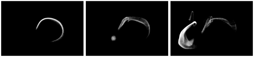
- Two examples of a simple reaction

_click.jpg)
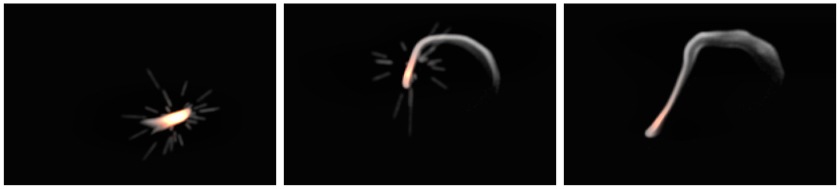
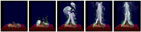
- Generation of gas-phase explosion-like effects using a simple reaction
_click.jpg)
- Generation of gas-phase explosion-like effects using a chain reaction
_click.jpg)
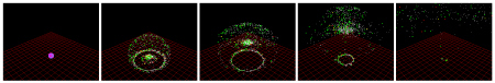
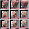
- Three examples of catalysis. The ball moving in a closed room behaves as a catalyst
_click.jpg)
.jpg)
.jpg)
.jpg)
.jpg)
- Image 1: [first row], [second row]
- Image 2: [first row], [second row], [third row], [fourth row], [fifth row]
- Image 3: [first row], [second row], [third row]
- Image 4: [first row], [second row], [third row]
- Not in the paper: [0], [1], [2], [3], [4], [5]